Michael Nielsen built RMNIST — MNIST with the training set cut down to 1, 5 or 10 examples per class — to ask a question he put plainly: people learn to recognise digits from a handful of examples, so what principle are we missing? He published baselines and left the problem open.

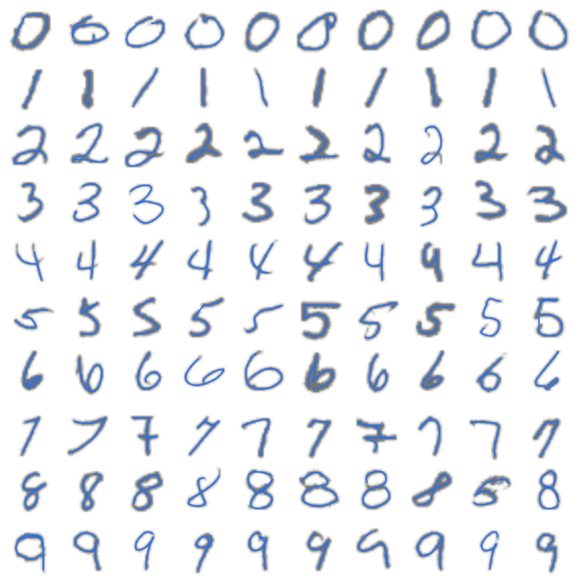
Here is one answer. I wrote a differentiable renderer that draws a digit as a single pen stroke: a spline with six control points, pushed through translation, rotation, scale, shear, truncation and a mild warp, and inked with a variable-width brush. Twenty-nine parameters. I fit it to each training image by gradient descent, which gives one little program per image. Then I classify a test image by fitting all of those programs to it and asking which class could get there most cheaply.

on 200 held-out test digits	RMNIST/1	RMNIST/5	RMNIST/10
best baseline (Nielsen)	0.569	0.844	0.921
this	0.825	0.935	0.960

Nielsen’s best numbers are a small convnet, with ±1 pixel translation augmentation where that helped (on RMNIST/1 it didn’t; ±2 pixels got him to about 0.60). His are measured on 10,000 validation images; mine on 200 test digits, so mine carry a standard error of about 1.5 points — treat the RMNIST/10 gap as real but not precise, and the RMNIST/1 gap as the interesting one.

Why you should not care about MNIST

The obvious dismissal is that I hand-wrote a generative model for the one domain where that is easy, and of course it wins. Half of that is right. Nobody hand-writes a renderer for cats. This is a toy, the toy was chosen because it is tractable, and the result does not transfer to anything by itself.

The part that isn’t toy is where the information came from, because it didn’t come from any of the usual places.

The idea in one picture

Fitting is unsupervised. The labels are used only afterwards, to group the fitted programs into ten piles. Classification is then: run the optimiser from each template and see which one can explain the image.

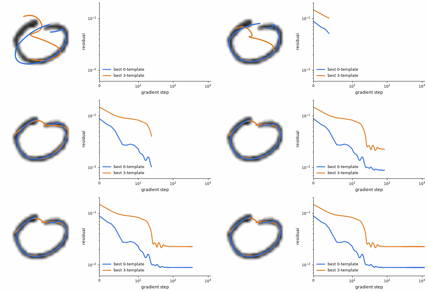
The 3-template is allowed to translate, rotate, scale, shear and bend. It gets a long way. It still cannot close the loop, and it pays for every pixel it moved — the fit is anchored, so the score is not “how well does this end up fitting” but “how far did this program have to travel”. A 0 is cheap to reach from another 0 and expensive to reach from a 3, and that is the whole classifier.

Three things worth knowing

The optimisation is doing the work, not the templates. If I skip the fitting and just compare the test image to the rendered templates pixelwise — the same hundred programs, used as prototypes — I get 0.695 instead of 0.960. The templates are not good pixel prototypes. They are good starting points.

The way you pool over a class matters more than what you measure. Averaging the cost over all ten templates of a class gives 0.925; averaging the best two gives 0.960. Handwriting style is multi-modal, and the mean drags in nine irrelevant styles to vote on every digit. On RMNIST/5 the ordering of the pooling rules is different again, which is a warning: I am choosing one of four rules on 200 digits, and that is worth about a point of the headline.

I expected the trajectory to carry information, and it didn’t. I scored by the total energy along the descent path, on the theory that a hard fit is a long climb. It correlates with the final residual at r = 0.9997, and the final residual alone does just as well. Nice idea, no effect.

The failures are also informative, and they are not failures of the measure. In 11 of the 15 digits that the mean rule gets wrong, the true class’s best template visibly fits better than the one that wins — the right answer is sitting there in the fits and gets averaged away. You can page through them; the full RMNIST/10 study, with the anchor sweep and the confusion matrix, is here.

A note on honesty, since small test sets invite self-deception: three separate times a setting that won on 200 validation digits failed to transfer to test — a pose-weighted anchor, a staged fit, and a tuned blend of energy and residual all looked like wins and weren’t. The only thing tuned for the numbers above is the anchor strength, on 40 validation digits.

What I actually think this is about

Nothing here learned a feature. There was no discriminative objective, no pretraining, and 100 images. What did the work is a model of how the image was made, plus the ability to run it backwards.

Once you can ask “what parameters would have produced this?”, you get a distance between images for free, and it is a distance with structure built in. It knows a rotated 7 is a 7 — not because it saw rotated 7s, but because rotation is a knob. That is a different kind of generalisation from the statistical kind: it holds where the data doesn’t go, because it was never estimated from data in the first place. It also knows when it is lost. A program that cannot reach an image says so, loudly, in units of residual.

Those properties aren’t properties of MNIST. They’re properties of having a causal model of image formation and being able to invert it. Which is why I think this is worth more than a cute benchmark result: we are suddenly quite good at learning simulators — video models, neural rendering, learned physics — and if you can learn one, inverting it at test time gives you the same free metric, the same explicit pose, and the same ability to refuse. The supervision budget goes to learning how the world makes images, which needs no labels, instead of to learning a mapping from images to one particular set of labels.

What would break first: inverting a learned simulator is slow, non-convex, and its latent knobs are not disentangled the way my seven transforms are. My optimisation works because the parameters mean something — half a day of design went into making translation cheap and knot-shuffling expensive. That is the hard part, and this post is not evidence that it is solvable. It is a demonstration that the payoff is worth chasing when the simulator is good.

Cost, for the record: about 0.2 seconds per test image on one GPU, for a hundred fits of 1200 gradient steps each. Expensive compared to a forward pass through a convnet, and all of it at test time rather than training time, which I suspect is the right place for it to be.