• Why you should not care about MNIST
• Classification by how far a program has to travel
• Thirteen distribution shifts, and where it breaks
• Learning simulators we can invert

Michael Nielsen built RMNIST - MNIST with the training set cut down to 1, 5 or 10 examples per class - to ask: people learn to recognize digits from a handful of examples, so what principle are we missing? He published baselines and left the problem open.

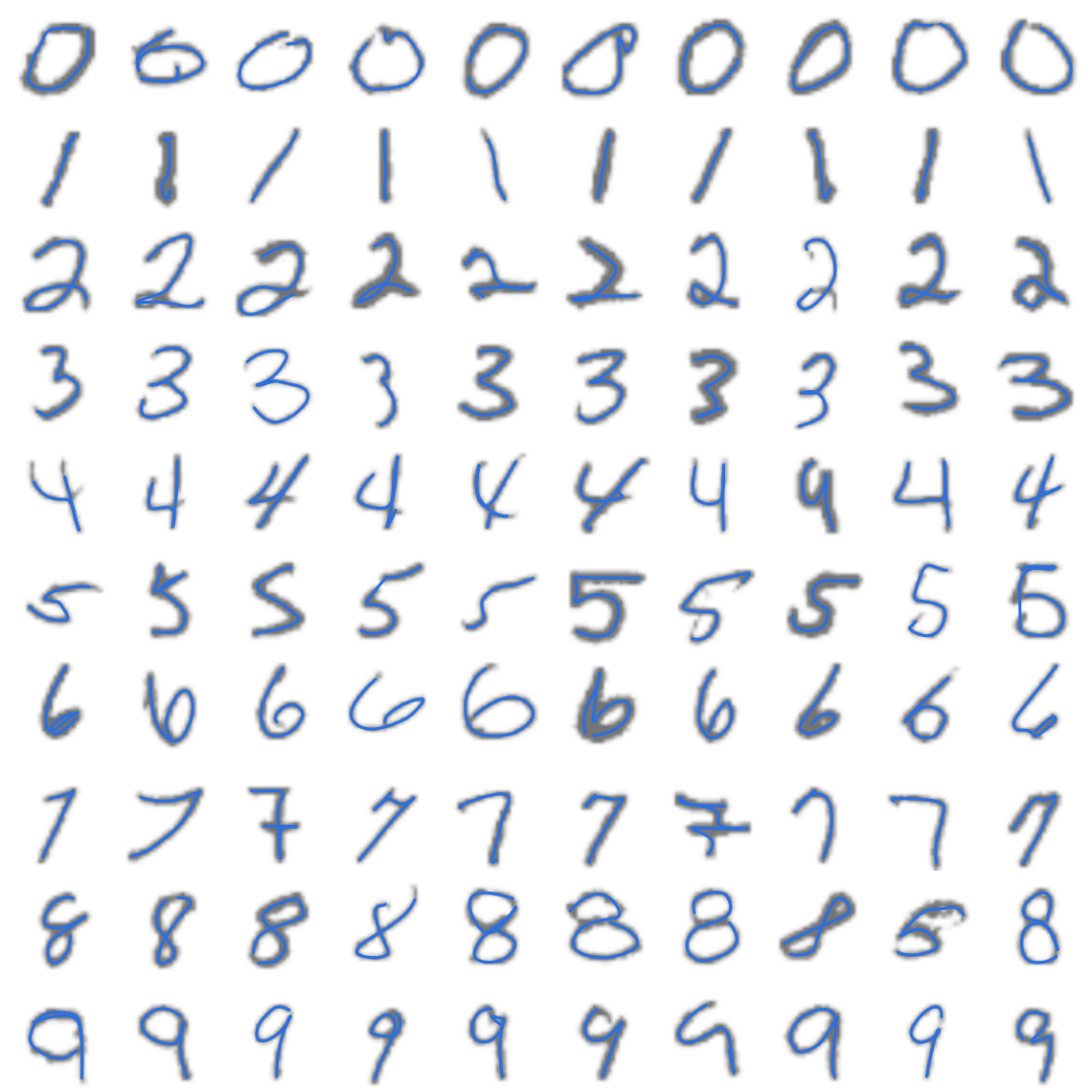
Here is one answer. I wrote a differentiable renderer that draws a digit as a single pen stroke: a spline with six control points, pushed through translation, rotation, scale, shear, truncation and a mild warp, and inked with a variable-width brush. Twenty-nine parameters. I fit it to each training image by gradient descent, which gives one little program per image. Then I classify a test image by fitting all of those programs to it and asking which class could get there most cheaply.

on 200 held-out test digits	RMNIST/1	RMNIST/5	RMNIST/10
best baseline (Nielsen)	0.569	0.844	0.921
this	0.825	0.935	0.960

Nielsen’s best numbers are a small convnet with ±1 pixel translation augmentation. His are measured on 10,000 validation images, mine on 200 test digits, so mine carry a standard error of about 1.5 points. The interesting number is RMNIST/1 - inverse rendering can one-shot learn MNIST pretty well, with zero pretraining.

Why you should not care about MNIST

As everyone knows, everything works on MNIST. Linear SVMs work on MNIST. A drug-addled, lobotomized rainworm works on MNIST. Communism works on MNIST. Clearly, I hand-wrote a generative model for a domain where the inductive bias fits perfectly, and there’s not much else going on in the image. Of course it wins. Nobody hand-writes a renderer for cats (though it works great for worms). In contrast, CNN + augmentation has much weaker inductive biases, and can learn a much broader range of data, given labels. But here, no labels were used to fit anything, and nothing learned a feature; it’s not quite a digit simulator, but it’s close - and it can be fit to data at test time.

Classification by how far a program has to travel

Fitting is unsupervised. The labels are used only afterwards, to group the fitted programs into ten piles. Classification is then: run the optimizer from each template and see which one can explain the image.

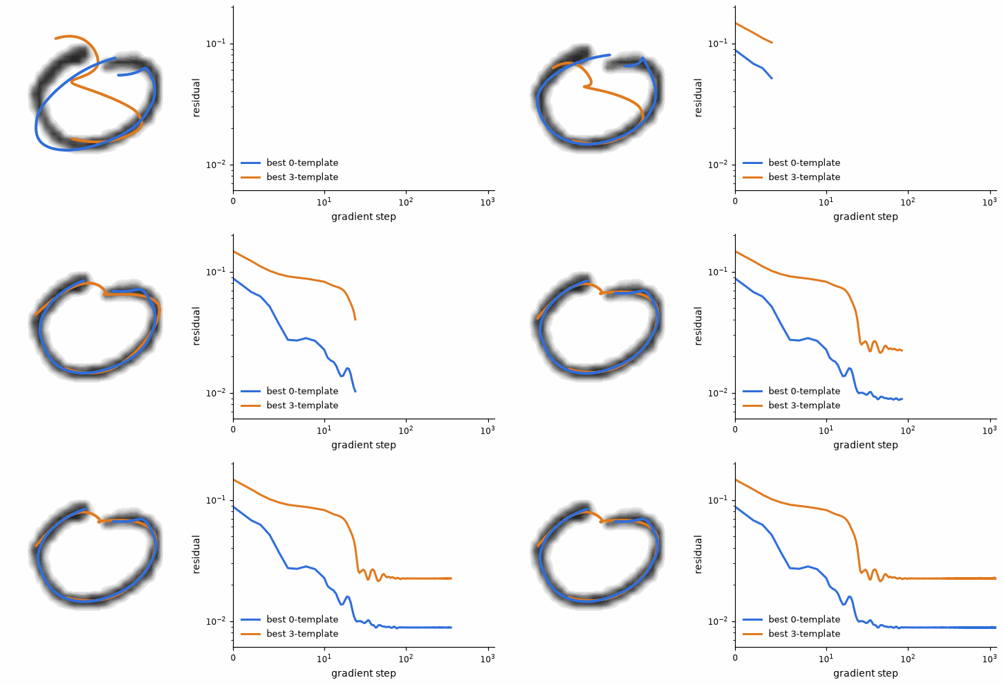
The 3-template is allowed to translate, rotate, scale, shear and bend. It gets a long way, but it still cannot close the loop. A 0 is cheap to reach from another 0 and expensive to reach from a 3, and that is the whole classifier. It turns out that whether you classify by how much work the optimizer had to do (the descent trajectory) or by the final residual, the results are the same. If a digit fits well, it was easy to make it fit.

The cost is about 0.2 seconds per test image on one GPU, for a hundred fits of 1200 gradient steps each. Expensive compared to a forward pass through a convnet, and all of it at test time rather than training time.

Importantly, it’s the optimization doing the work, not the training templates. Comparing a test image to the rendered templates pixelwise - the same hundred programs, used as prototypes - gives 0.695 instead of 0.960.

How you pool over a class matters. Averaging the cost over all ten templates of a class gives 0.925, averaging the best two gives 0.960. Handwriting style is multi-modal, and the mean drags in nine irrelevant styles to vote on every digit. Often, the true class’s best template fits better than the (mistaken) winner - the right answer is sitting in the fits and gets averaged away. You can page through them, or see the full study.

Thirteen distribution shifts, and where it breaks

If this works because the model has knobs for the ways a digit can vary, it should generalize out of distribution: survive those variations without having been shown any. Thirteen corruptions, 1000 held-out test digits, three fixed models: the spline fitter, a faithful port of Nielsen’s convnet - reproduced at 0.914 ± 0.004 against his 0.921 - and that convnet retrained with rotation and scale augmentation at exactly the magnitudes tested, which hands it the answer in advance.

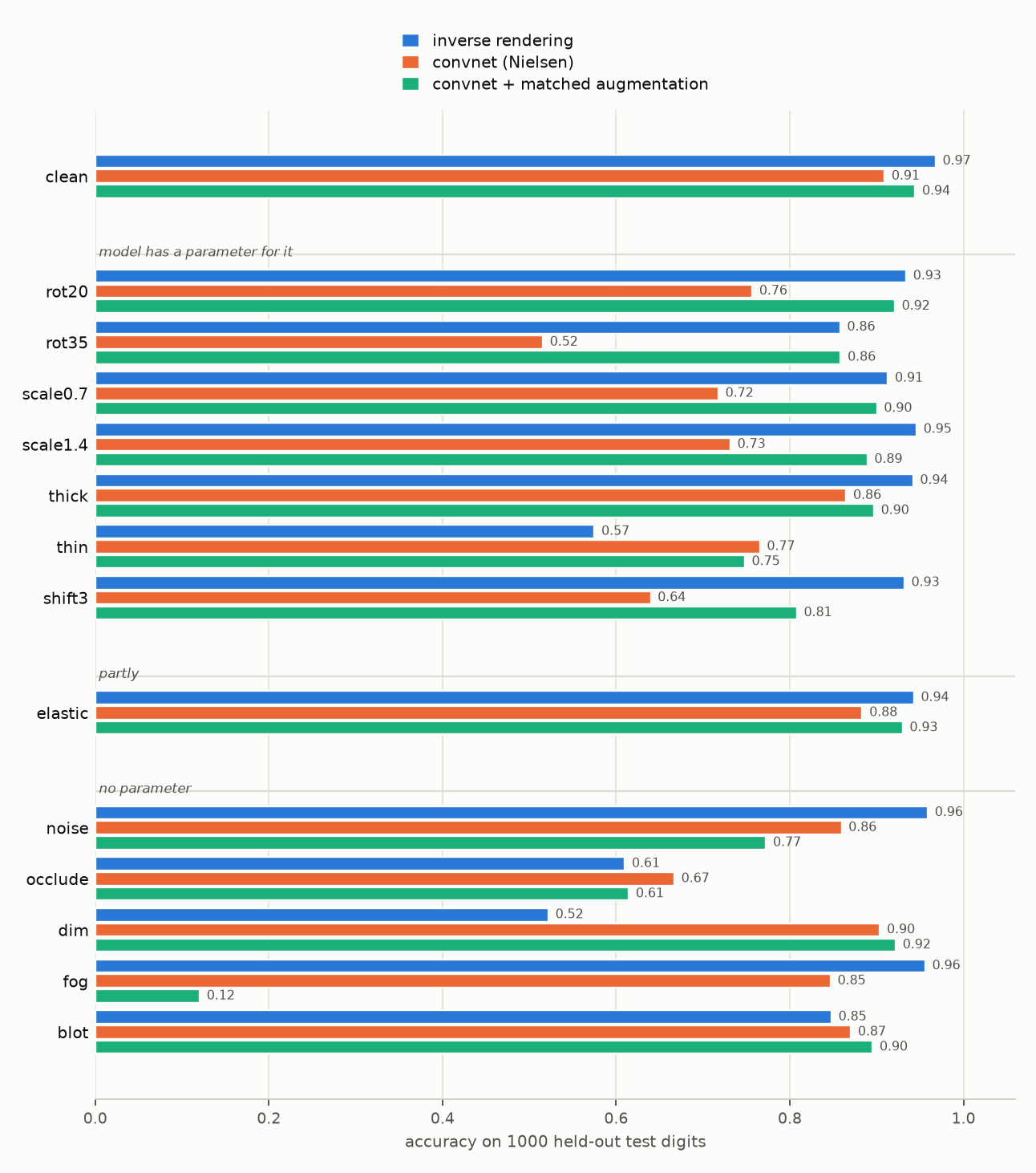
Where the renderer has a parameter, it holds up. Rotate by 35° and the convnet falls to 0.52 while the fitter, told nothing, keeps 0.86. Shift by three pixels: 0.64 against 0.93. The augmented convnet recovers on the geometry it was augmented for, as it must, and pays for it elsewhere: teaching it rotation and scale cost it nine points on additive noise and, on a uniformly raised background, collapsed it to 0.12, where it answers “8” to 906 of 1000 digits.

But having a knob turns out not to predict robustness. Thinning the strokes is a knob - the brush has a width parameter, and it does adapt - yet accuracy falls to 0.58, the worst of the three. Dimming the ink to 45%, which the renderer genuinely cannot express, is worse still at 0.52, while both convnets barely notice. A raised background is equally inexpressible and costs the fitter nothing at all.

The reason is not in the renderer but in the objective. The data term is a flat mean squared error over every pixel, ink and background alike. For a thinned digit, rendering a blank image scores 0.021 and rendering the correct digit scores 0.043 - the fit is not getting stuck, it is converging on what I actually asked for. I could have fiddled with loss, and tried to make it robust to this failure mode. As a digit simulator, this one is imperfect, and would remain imperfect if I fixed that flaw. The point is, it can adapt in circumscribed ways, and fail in other ways - generalization depends on the quality of the explanation it encodes and navigating the optimization landscape. This is very different from an NN, which can learn an invariance if the right augmentation is provided at training time, but won’t adapt at all at test time - there, generalization mainly depends on the training data distribution.

Small test sets invite self-deception, and three separate times a setting that won on validation - a pose-weighted anchor, a staged fit, a tuned blend of energy and residual - failed to transfer to test. The only thing tuned for the numbers here is the anchor strength, on 40 validation digits.

Learning simulators we can invert

What did the work is a model of how the image was made, plus the ability to run it backwards. No discriminative objective, no pretraining, a hundred images.

Once you can ask “what parameters would have produced this?”, you get a distance between images for free. It knows a rotated 7 is a 7 - not because it saw rotated 7s, but because rotation is a knob. That knob isn’t there to survive rotated test digits; it is there because that is how ink gets onto paper, and the invariance is a by-product.

That is a different kind of generalization from the statistical kind: you stop having to guess the test distribution and start having to get the data generating process right instead. And you know if you get it wrong, which may be the more valuable half - a simulator that cannot generate an image says so, loudly, in units of residual.

Those are properties of having a causal model of image formation and being able to invert it, not properties of MNIST. Which is why I think this is about more than sample efficiency. We are getting very good at learning neural simulators: video models, neural rendering, learned physics. We also have mature fields involved in inverting handcrafted simulators - inverse problems in the natural sciences, probabilistic programming, inverse graphics. But we haven’t figured out how to learn simulators represented as code, which can be fit to real data, in real time.

That’s where I think this is going, with little evidence yet (coming soon to a google scholar page near you): not a replacement for deep learning, not a return to handcrafted models in a stubborn denial of the Bitter Lesson, but a division of labor among three components that complement each other. An NN that proposes the initial parameters, trained on samples from the current simulator. A simulator we can invert, fitting real data, and providing training data for the NN. And a coding agent that adapts the simulator when it cannot explain what it is looking at.

Why would this work? In large part, it already does work. Deep learning works on anything given enough data and the right architecture. With simulators, we have infinite data, but so far, the sim2real gap, the divergence between a simulator and the real data distribution, has hamstrung the approach. Inverse problems are the backbone of physics, geology and many engineering fields. But they are notoriously difficult to solve, mainly because of local minima - for anything more complex than drawing single curved lines, you need a guess for the initial parameters that lands you pretty close to the right answer. We’re already using NNs to mitigate, or “amortize” this, both for inverse problems and probabilistic programs. Finally, coding agents clearly work - Claude wrote all the code I’m using here - given the right guidance. We know they can do incredible things given the right learning signal - such as solve longstanding problems in math given proof assistants that verify their attempts. We don’t have verifiers for vision, or motor control, or biology. But we have renderers, ODE solvers, SAT solvers, physics engines, and tons of other existing machinery for expressing and solving inverse problems. Why don’t we put them to work?