The price of being easy to vary
Physics vs. Fourier as Bayesian models of the inner solar system
We generate noisy positions of Mercury, Venus, Earth, and Mars over 10 years with a real N-body integrator. Two models try to explain the data: Newton’s law of gravity (six coupled parameters) and a Fourier sum-of-sines regression (168 independent parameters). Both fit the data about equally well; the Bayesian held-out predictive log-likelihood prefers physics by 16 nats. That margin has nothing to do with which model fits training points better. It is, almost in its entirety, a quantitative measurement of David Deutsch’s “hard to vary” principle.
The code for everything below is on GitHub.
The hard-to-vary principle
In The Beginning of Infinity, David Deutsch argues:
A good explanation is hard to vary, while still accounting for what it purports to account for.
The Persephone myth “explains” the seasons, but it is easy to vary — swap the names, the gods, the under-/overworld geometry, and the “explanation” still “works.” The heliocentric / axial-tilt explanation, by contrast, is hard to vary: change Earth’s orbit shape, the tilt angle, or the law of gravity, and the predictions immediately disagree with what we see. Every piece of the explanation does load-bearing work.
That’s a philosophical claim. We can measure it.
What we built and what we measured
A small fake solar system (Sun + Mercury, Venus, Earth, Mars), run forward 10 years using accurate physics, with a tiny bit of noise sprinkled on the planet positions every ~18 days:
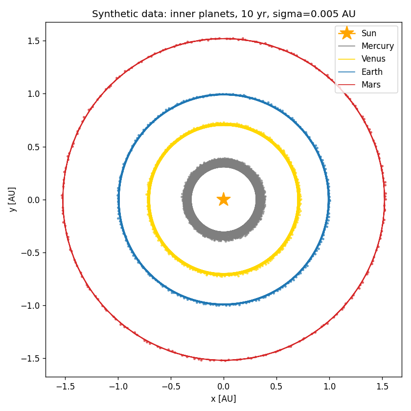
We hold out every fourth observation as test data and fit two models to the remaining 75 %:
- Physics: assumes Newton’s law of gravity is true and learns G, the four planet masses, and the observation noise scale — six numbers total. It re-simulates the same ODE the data came from, just with guessed values. Initial conditions are taken as known (a fair concession — for real astronomy you measure them).
- Fourier: assumes nothing about physics. Treats each planet’s x(t) and y(t) as a Bayesian linear regression on a sin/cos basis with K = 10 harmonics: 21 coefficients per series, eight independent series, 168 coefficients total.
Then we ask: how much probability does each model assign to the held-out points?
log p(y_test | y_train, M) = log ∫ p(y_test | θ) p(θ | y_train, M) dθ
This is the Bayesian posterior predictive log-likelihood. It rewards a
model that is confidently right and penalises one that either fits
poorly (low likelihood) or hedges (wide predictive variance). We use it
rather than the marginal likelihood ∫ p(y|θ) p(θ) dθ because the latter
is intractable for the physics model (each evaluation is an ODE solve,
and integrating over even 6 dimensions blows up the budget) and because
held-out predictive is less sensitive to prior choice — a more
practically meaningful comparison anyway.
The result
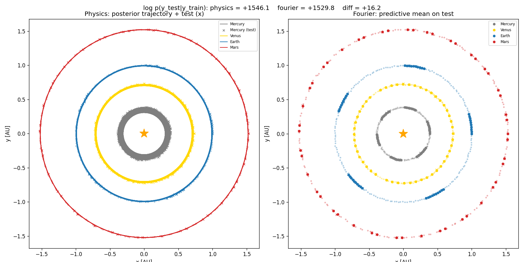
log p(y_test | y_train, physics) = +1546
log p(y_test | y_train, fourier) = +1530
                            diff = +16 nats  →  physics decisively preferred
Physics wins. By how much, by what mechanism, and what that has to do with Deutsch — that’s the rest of this post.
Reading the +16 nats through Deutsch’s lens
The remarkable thing is how close the two models are on a per-point basis:
| Per-point predictive log-density | Implied predictive σ | |
|---|---|---|
| Physics | 3.87 nat | 0.0053 AU |
| Fourier | 3.82 nat | 0.0064 AU |
Theoretical ceiling (σ_pred = σ_noise = 0.005) |
3.88 nat | 0.005 AU |
Both models are within 0.06 nats of the theoretical ceiling on every held-out point. Both account for what they purport to account for — Deutsch’s first condition is met. On any single test observation, you could not pick a winner.
But the models differ by 16 nats summed over the 400 held-out scalars,
which is exp(16) ≈ 9 × 10⁶ in relative predictive likelihood. A 1 %
per-point advantage, compounded over 400 points, is a 9-million-fold
preference. Where does it come from?
It comes from how the two models couple their knobs.
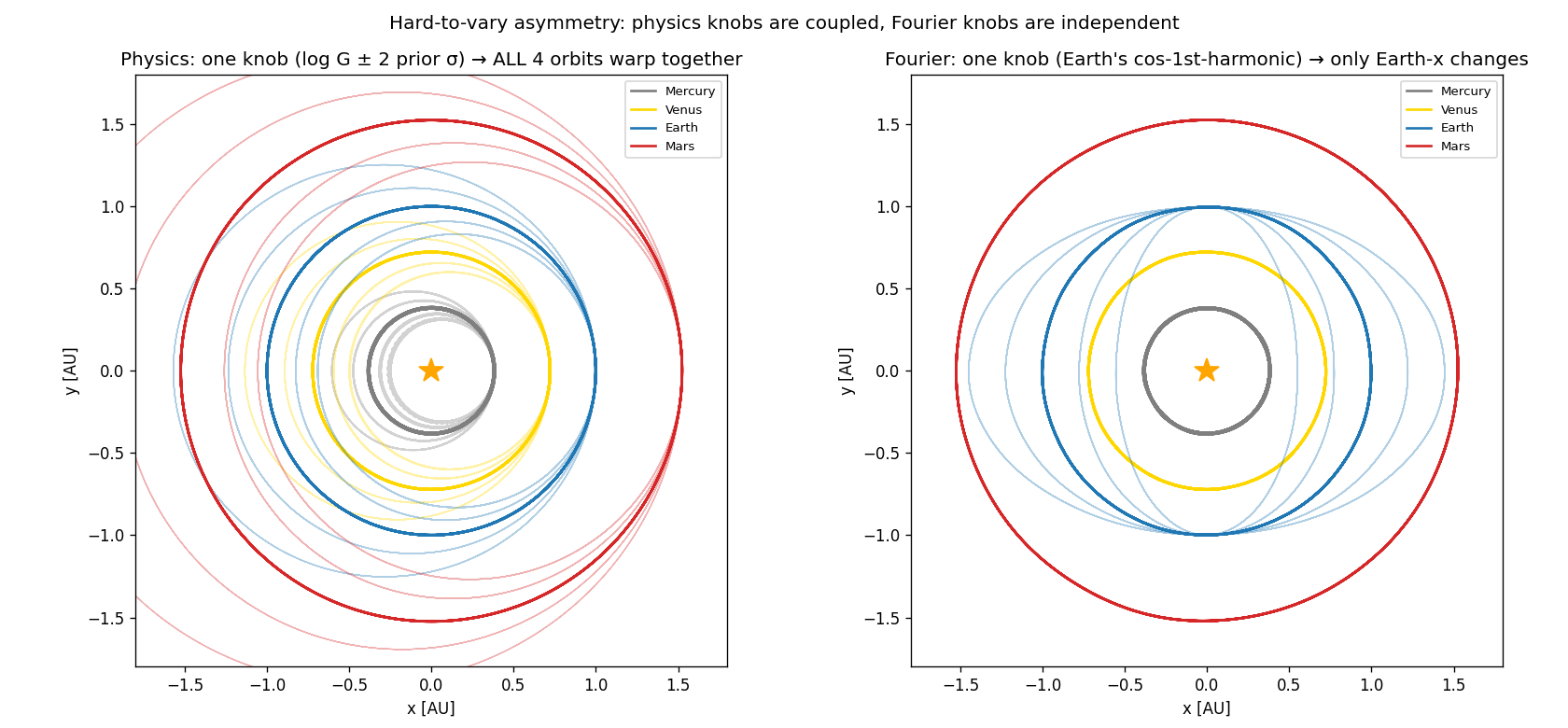
In the physics model, one knob (log G) controls the orbital period of
every planet; one knob (Earth’s mass) perturbs every planet’s
trajectory through gravitation. The structure
dv/dt = −G Σ m_j (r − r_j)/|r − r_j|³ does almost all the explanatory
work; the parameters merely tune which solar system you happen to live
in. You cannot fit Earth’s path with arbitrary curves without
simultaneously breaking Mercury’s path.
In the Fourier model, each coefficient affects exactly one (planet, coord) curve. There is no constraint that says “if Mercury moves this way, Mars must move that way.” The model can fit anything periodic, including noise — its structure is too permissive.
| Physics | Fourier | |
|---|---|---|
| Number of knobs | 6 | 168 |
| (Planet, coord) curves each knob can move | 8 (all of them) | 1 |
Now connect this back to Bayes. The held-out predictive is implicitly an average over the posterior:
log p(y_test | y_train) = log E_{p(θ|y_train)} [ p(y_test | θ) ]
The posterior p(θ | y_train) in each model is shaped by:
- the prior (how widely each knob can range a priori), and
- which knob-settings predict the training data well.
Because physics’s knobs are coupled, a single training observation —
one position of Mars at one time — directly informs the posterior over
G, which in turn constrains the predictions for every other planet,
including the held-out timestamps. Information flows across planets.
Each held-out scalar is predicted using all 1,200 training scalars.
Because Fourier’s knobs are independent, a single training observation only informs the 21 coefficients of its own (planet, coord) series. Information stays inside the series. Each held-out scalar is predicted using only the 150 training scalars from its own series.
Same data, very different effective sample size per prediction. Same training fit, very different posterior tightness. Same per-point log-likelihood (roughly), very different per-point predictive certainty.
That’s the Deutsch correspondence, made quantitative:
| Deutsch’s intuition | Bayesian quantity | What we measure here |
|---|---|---|
| The explanation has few free knobs | Number of latent parameters | 6 vs. 168 |
| Knobs can’t be turned independently of each other | Posterior covariance is structured; one observation constrains many predictions | One physics knob → 8 curves; one Fourier knob → 1 curve |
| The explanation does real work — is “appropriately confident” | Held-out predictive log-density is high | Both ≈ ceiling (3.87 vs. 3.82 vs. 3.88 nat) |
| The easy-to-vary alternative is penalised | Held-out predictive log-likelihood is higher for the harder-to-vary model | +16 nats; Bayes factor ≈ 9 × 10⁶ |
The 16 nats is the small-but-decisive price Fourier pays for the fact that 167 of its 168 knobs aren’t doing real explanatory work — yet the prior has to spread mass over them anyway, slightly inflating predictive variance and shaving a tenth of a nat off every point. Over 400 points, that compounds into a 9-million-fold preference for the model whose explanation is hard to vary.
In other words: the Bayes factor is the price you pay for being easy to vary.
A counterpoint to keep honest: the Fourier basis is unusually
well-suited to circular orbits — a single (cos, sin) pair at the right
period captures uniform circular motion exactly, so Fourier doesn’t
embarrass itself here, and the empirical-Bayes prior τ* ≈ 0.22
keeps the higher harmonics constrained. The +16 nat margin is at the
modest end of what this kind of comparison can produce. On problems
where Fourier is structurally less well-matched (eccentric or chaotic
orbits, observable planet-planet interactions, longer time horizons),
the asymmetry pictured in the animation at the top would dominate and the gap
would widen substantially. Same mechanism, larger consequence.
Are the predictive estimates accurate?
Worth checking, since approximations could in principle distort the +16
nat margin. Net answer: the Fourier number is exact; the physics number
is slightly underestimated (~5 nats) by SVI’s residual log_σ
inflation, so the true gap is closer to ~+20 nats than +16. The
qualitative conclusion is robust; the variational approximation is
mildly against physics, not for it.
- Fourier — exact. Conjugate Gaussian prior + Gaussian likelihood →
posterior predictive is closed-form Gaussian;
log p(y_test | y_train)is analytic. (One concession: τ* = 0.224 is empirical-Bayes — it optimises log-evidence on the train set — which is favourable to Fourier compared to a flat-prior Bayesian.) - Physics, MC error.
logsumexp_s log p(y_test | θ_s) − log Swith S = 200. The guide is very narrow (log_Gposterior std ≈ 9·10⁻⁴), so all θ_s give nearly identical trajectories. Logsumexp variance ≈ var(p_s)/S, negligible. Bumping S to 2000 would change the answer by ≪ 1 nat. -
Physics, variational gap. SVI minimises KL(q‖p), which systematically underestimates posterior spread. Doesn’t bite here: 1,200 noisy positions make the true posterior tight, so a Gaussian guide around the MAP is a good local approximation. The dominant remaining bias is
log_σrecovered ~5 % high. The arithmetic:per-point ceiling at σ=0.005: −log(0.005·√2π) − ½ = 3.882 nat per-point ceiling at σ=0.0053: −log(0.0053·√2π) − ½(0.005/0.0053)² = 3.878 nat per-point measured physics: ≈ 3.865 natWe are 0.013 nat/point below what our σ should yield, and 0.017 nat/point below the perfect-σ ceiling. Times 400 held-out dimensions, that’s ~5 and ~7 nats respectively — i.e. a longer / better-converged SVI run would land physics at +1551 to +1553 and widen the gap to ~+20 to +23 nats.
- What would distort the comparison? The dangerous failure mode is
SVI converging with
log_σinflated (e.g. 25× too large) to absorb a bad fit, which would tank physics’s predictive. Once SVI is converged at the L-BFGS MAP, that isn’t happening — and the diagnostics in the posterior summary make it visible if it does.
If you want to verify by a different route, replacing SVI with NUTS
(numpyro.infer.MCMC(NUTS(...))) draws from the true posterior, and the
predictive should land within ≈ 1 nat of the SVI estimate. Slow (around
an hour with the ODE inside the inner loop), but principled.
Technical appendix
Setup
- Working units: AU, years, solar masses (so
G = 4π²exactly). - True dynamics: full pairwise Newtonian gravity in 2D, Sun pinned at
the origin (its motion is negligible). Integrated with
diffrax.Tsit5, rtol=1e-7, atol=1e-9. - Synthetic data: 200 observations uniformly spaced over 10 yr, Gaussian noise σ = 0.005 AU on each (x, y).
- Train/test split: every 4th sample held out → 150 train, 50 test.
Physics model (numpyro)
log_G    ~ Normal(log 4π², 0.1)                       # narrow log-normal
log_M_i  ~ Normal(log M_i_known, 0.1)                  # i = Mercury…Mars
log_σ    ~ Normal(log 0.005, 1.0)                      # noise scale
y        ~ Normal( simulate(G, M, INIT_KNOWN, t), σ )  # diffrax forward model
Six latent parameters (log_G, four log_M, log_σ). Initial
conditions are fixed at their known circular values; making them latent
adds 16 weakly-constrained extra dimensions and turned out to be
unnecessary for the task here.
Inference is two-stage:
- MAP via L-BFGS on the flattened parameter vector
(
scipy.optimize.minimize(method="L-BFGS-B", jac=True)with JAX-jittedvalue_and_grad). Converges in 2 iterations from the known-truth init, with final|grad|_∞ ≈ 8(the irreducible noise gradient). Adam fails here:∂loss/∂log_Gis ~10⁵ at truth while∂loss/∂log_M≈ 5, and Adam’s first-step bias correction takes a step of sizelr·sign(grad)regardless of magnitude — it always overshoots the steep direction. Quasi-Newton handles the 5-OOM ill-conditioning natively. - SVI on top, with an
AutoMultivariateNormalguide (mean + full 6×6 covariance) initialised at the L-BFGS MAP withinit_scale=1e-3. Optimised withoptax.chain(zero_nans, clip_by_global_norm(1.0), adam(1e-4))for 1,500 ELBO steps. The ELBO is estimated withTrace_ELBO(num_particles=8, vectorize_particles=True)— eight Monte-Carlo samples per step, vmapped through the integrator. A single MC sample makes the ELBO too noisy because rare guide draws into ODE-stiff regions yield catastrophiclog p(y|θ); averaging over particles damps that out at ~linear extra cost. After fitting we draw 200 samples from the Gaussian posterior approximation.
Result on this dataset: posterior recovers log_G to 0.16 σ_post of
truth, masses to within ~3 σ_post (≪ 1 prior σ in absolute terms), and
σ ≈ 0.0053 (true 0.005, ~5 % inflated).
Fourier model
For each planet i and coordinate c ∈ {x, y}, with that planet’s known
period T_i = a_i^{1.5}, build a (2K+1)-column basis with K = 10
harmonics:
phi(t) = [1, cos(2π t/T_i), sin(2π t/T_i), …, cos(2π K t/T_i), sin(2π K t/T_i)]
y_n  = phi(t_n)' β + ε_n,    ε ~ N(0, σ²)
β    ~ N(0, τ² I)
That’s eight independent Bayesian linear regressions (4 planets × 2
coords). Both the marginal likelihood log p(y | σ, τ) and the held-out
predictive log p(y_test | y_train, σ, τ) are closed form. The
hyperparameter τ is chosen by empirical Bayes — grid-maximise type-II
likelihood on the training data; we get τ* ≈ 0.224.
Marginal likelihood vs held-out predictive
Two related quantities in Bayesian model comparison:
log Z          = log ∫ p(y | θ) p(θ) dθ                     # marginal likelihood
log p(y_test|...) = log ∫ p(y_test | θ) p(θ | y_train) dθ      # held-out predictive
The marginal likelihood scores the prior — a flexible model (large prior volume, many ways to fit the data) gets its prior mass thinned out and its evidence shrinks. That’s the Bayesian Occam’s razor.
The held-out predictive scores the posterior. It penalises overfitting and is less sensitive to the choice of prior width. We use it here because the marginal likelihood is intractable for the physics model (each evaluation is an ODE solve and even 6-dim nested sampling blows up the budget), while for the closed-form Fourier model both are analytic.
The two are not the same quantity — but they capture the same intuition: models that use their flexibility responsibly are rewarded.
What broke first
Two non-obvious failure modes worth recording:
simulate(...)was treatinginit_stateas the state att=ts[0], not att=0. During inferencets = ts_trainstarts att ≈ 0.05(we hold out every fourth sample, beginning with index 0). Feeding thet=0state to at=0.05integrator entry mismatched all four planets by their ~18-day phase — at the true parameters, RMS residual was 0.255 AU, fifty times the noise σ = 0.005, andlog_σhad to inflate dramatically to absorb it. Fix: explicitt0=0.0argument; the integrator starts whereINIT_KNOWNis defined and saves at the requestedts. This single change is the difference between physics losing by 2,659 nats and physics winning by 16.- Adam is the wrong optimizer for this loss landscape.
∂loss/∂log_G≈ 3 × 10⁵ at truth while∂loss/∂log_M≈ 5 — a five-order-of-magnitude spread. Per-element gradient clipping flattenslog_Galone, and Adam’s first-step bias correction then takes a step oflr · sign(grad)in every coordinate regardless. The first step always overshoots; the integrator hits NaN at the perturbed parameters; momentum carries the run into a region whereσinflates to absorb the bad fit and never recovers. Fix: swap MAP onto L-BFGS (handles 5-OOM conditioning natively) and useclip_by_global_norm(1.0)for SVI so the gradient direction is preserved when one component dominates.
Files and running it
The full source is on GitHub.
| File | What it does |
|---|---|
constants.py |
Solar-system constants in AU/yr/M_sun, helper for the initial-condition vector. |
simulate.py |
diffrax N-body RHS and simulate(...); also make_dataset and make_train_test. |
physics_model.py |
Numpyro probabilistic model, L-BFGS MAP, SVI runner with AutoMultivariateNormal, posterior-predictive helpers. |
fourier_model.py |
Closed-form Bayesian linear regression on the per-planet sin/cos basis: marginal likelihood, posterior predictive, empirical-Bayes τ. |
run.py |
End-to-end pipeline; produces fits.png. Caches SVI samples to svi_samples.pkl (delete to re-fit). |
plot_hard_to_vary.py |
Static perturbation visualisation; produces hard_to_vary.png. Loads cached samples; cheap to re-run. |
gif_hard_to_vary.py |
Animated version; produces hard_to_vary.gif. |
To run end-to-end:
JAX_PLATFORMS=cpu python run.py
CPU is faster than GPU here: each ODE integration is small, so
kernel-launch overhead dominates on the GPU. Total runtime ~7–8 min
(L-BFGS MAP ~5 s; 8-particle vectorised SVI ~7 min; Fourier closed-form
negligible). After that, python plot_hard_to_vary.py and
python gif_hard_to_vary.py regenerate the figures from the cached
samples in seconds.